This week, I tried to learn one of the most well-known Machine Learning methods, namely Linear Regression. (read the Indonesian version here) You know, lately Im very interested in Machine Learning. So, Im decided for learning this. There are 2 well-known learning model in ML, Supervised Learning and Unsupervised Learning. This algorithm is Supervised Learning. It means, we need some data (which called dataset) to train this algorithm to learn what to do.

The Linear Regression

So, what is Linear Regression ? Based on wikipedia, Linear Regression is a linear approach to modelling the relationship between dependent variable and independent variable. For example, the relation between age and weight, house area and price, etc. If you are remember the math lesson about The Equation of Straight Line in senior high school, we will use it here. In short, the formula is

1

y = mx + b

and the graph is

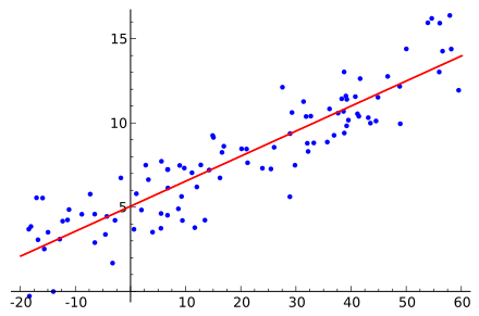
As I mentioned before, we have a dataset to train our algorithm. From the picture above, the dataset is the nodes around the tilted line. So, our work is find the tilted line based on the dataset. The question is, how ??

Gradient Descent

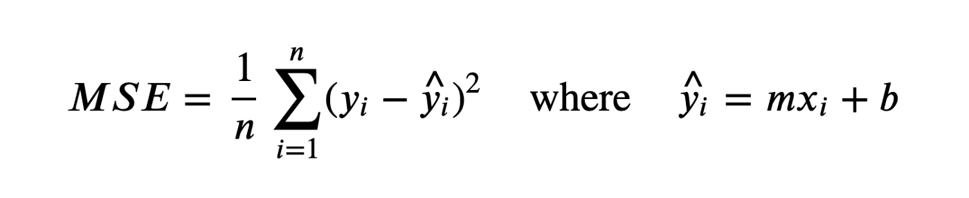
Gradient Descent is the way to find the line. From the formula above, we already have the pair of X and Y from our dataset. We will find the slope(m) and the intercept(b). The goal of the Gradient Descent algorithm is to find the line that comes closest to all these points. Once optimal parameters are found, we usually evaluate results with a Mean Squared Error (MSE). We remember that smaller MSE is better. In other words, we are trying to minimize it.

Derivatives

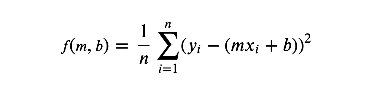
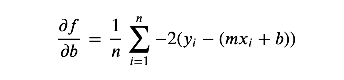
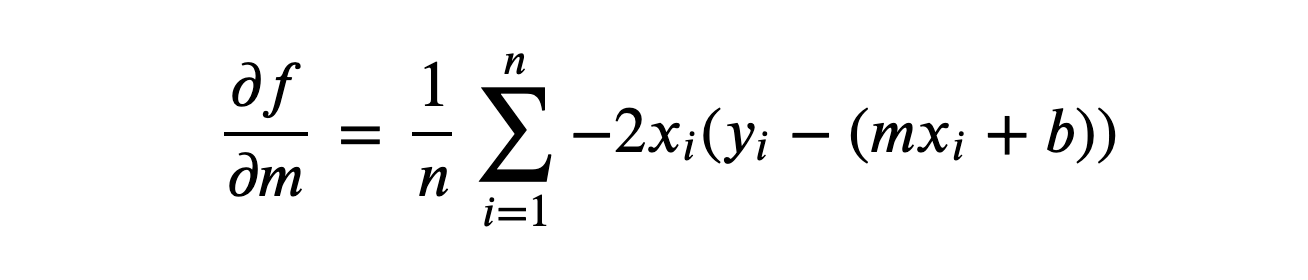
We use partial derivatives to find how each individual parameter affects MSE. We take these derivatives with respect to m and b separately. Take a look at the formula below. It is almost the same as MSE before, but this time we added f(m,b) to it. To get the partial derivatives we are going to use the Chain Rule. After calculating with Chain Rule, we get the partial derivative of MSE with respect to m Also, we get the partial derivative of MSE with respect to b We will use both of these functions to update m and n in each iteration of our algorithm, getting closer to our optimal line each time.

Lets Make Our Hand Dirty

You can find the code I’ve written here. First, lets make our data structure to manage the data used in function

1
2
3
4
5
6
7
8
9

// RegressionData for collecting some data that needed in linear regression calculation
type RegressionData struct {
	XValues      []float64
	YValues      []float64
	Epoch        int
	LearningRate float64
	slope        float64
	intercept    float64
}

The XValues will hold the x values from the dataset. YValues will hold the y values from the dataset. Epoch is the number of iteration. As mentioned before, the Gradient Descent need the iteration to find the best m and b. The LearningRate represents how fast our algorithm will learn with each iteration. By the way, I will use function with receiver. So I can get the data wherever it needed. This method will plot our dataset into the graph

1
2
3
4

// PlotTheDataset will make the scatter plot based on x and y values
func (d *RegressionData) PlotTheDataset() {
	d.plotMaker(false)
}

To get as close as possible to the optimal value for both m and n, we have to iterate until we reach epochs and update both values at each step

1
2
3

for i := 0; i < d.Epoch; i++ {
    d.slope, d.intercept = d.gradientDescent(d.slope, d.intercept)
}

The gradientDescent method is our actual algorithm. It will iterate through all the values of our input data (XValues and YValues) and update m and n using the derivates from above.

 1
 2
 3
 4
 5
 6
 7
 8
 9
10
11
12
13

func (d *RegressionData) gradientDescent(mCurrent float64, bCurrent float64) (finalM float64, finalB float64) {
	var mGradient float64
	var bGradient float64
	nData := len(d.XValues) //the x or y values length
	twoPerN := float64(2) / float64(nData)
	for i := 0; i < nData; i++ {
		mGradient += -twoPerN * d.XValues[i] * (d.YValues[i] - ((mCurrent * d.XValues[i]) + bCurrent))
		bGradient += -twoPerN * (d.YValues[i] - ((mCurrent * d.XValues[i]) + bCurrent))
	}
	finalM = mCurrent - (d.LearningRate * mGradient)
	finalB = bCurrent - (d.LearningRate * bGradient)
	return
}

Right after the loop, we use the LearningRate number to control slope and intercept. We don’t want our gradient over jump. Now lets input our number in the main package. We will use the static x and y values.

 1
 2
 3
 4
 5
 6
 7
 8
 9
10
11
12
13
14

func main() {
	xValues := []float64{1, 2, 3, 4, 5}
	yValues := []float64{1, 3, 2, 3, 5}
	lr := linearregression.New()
	lr.XValues = xValues
	lr.YValues = yValues
	lr.Epoch = 200
	lr.LearningRate = 0.05
	lr.PlotTheDataset()
	m, b := lr.Calculate(true)
	fmt.Println("m (slope) = ", m)
	fmt.Println("b (intercept) = ", b)
	fmt.Printf("so, the function is y(x) = %.2f x + %.2f", m, b)
}

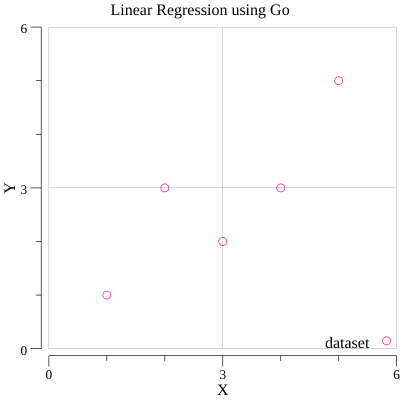
This is the graph after we plot our x and y values into it.

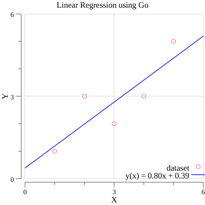
After calculating, we get the formula. y(x) = 0.80 x + 0.39 (with round 2 decimal). Lets plot this line formula into the graph.

That’s it. Feel free to check the source code and hit the star button if you like it. Let me know if you have the question. Just put it in the comment below. I will answer it as fast as I can. Thanks, see you.